Basic Usage
This package makes analysis of your image stacks easy. Here, we will walk through a basic example of analyzing a fresh image stack from start to finish.
Before beginning, ensure that the package is successfully installed (see Installation).
Capturing Images
During image capture, be sure to keep track of the strain of each animal. You will
need to know who is who during analysis. This is referred to as the strain indexer.
The software expects the strain indexer in the following format:
strain
start_animal
end_animal
HD233
1
100
SAY47
101
200
HD233
201
300
Organizing Files
Create a folder on your computer with the following format (we will refer to this as
the experiment ID):
YYYY_MM_DD-experiment_id
For example, let’s say we’ve imaged HD233 and SAY47 at 4mm levamisole. An appropriate experiment ID might be:
2019_02_26-HD233_SAY47_4mm_lev
Once the folder is created, save your image stack as experiment_id.tiff and
strain indexer as experiment_id-indexer.csv in that folder.
So in our example, we would save our image stack as 2019_02_26-HD233_SAY47_4mm_lev.tiff and our strain
indexer as 2019_02_26-HD233_SAY47_4mm_lev-indexer.csv.
Settings File
The pipeline requires multiple paramters be set. These parameters are specified in
the config file. To create a config file, navigate to your directory, then run the
pharedox create-settings command, like so:
$ cd /path/to/experiment/directory
$ pharedox create-settings
This will create a template configuration file, which you can customize to your liking.
Parameters
Here is an overview of the parameters used in analysis
pipeline
These parameters have to do with the image analysis
- strategy
a string that will help you identify which parameters you chose (for example,
reg). This will be appended to the date that you ran the experiment to create the name of the analysis directory.- channel_order
The order in which the images were taken. Should be a comma-separated list like so:
TL, 470, 410, 470, 410.- trimmed_profile_length
The vector length of the trimmed profiles
- untrimmed_profile_length
The vector length of the untrimmed profiles (how many points to be sampled along the midline)
- seg_threshold
The threshold used for segmentation. If
seg_images.ncis present in theprocessed_imagesdirectory, this is ignored.- measurement_order
The order of the spline for interpolation to use when measuring the images. The order has to be in the range [0, 5].
- measure_thickness
The width of the midline to measure under (pixels)
- reference_wavelength
The wavelength to use as a reference for rotation, midline generation, etc.
- image_register
Whether or not to register the images (experimental). 0=no, 1=yes
- channel_register
Whether or not to perform 1D channel registration on the profiles after measurement. 0=no, 1=yes
- population_register
Whether or not to perform 1D position standardization on the profiles after measurement. 0=no, 1=yes.
- trimmed_regions:
a mapping from region name to region boundaries. The trimmed profile data will be averaged within these boundaries for the summary statistics. Should look like this:
pm3: 0.07, 0.28
pm4: 0.33, 0.45
pm5: 0.53, 0.70
pm6: 0.80, 0.86
pm7: 0.88, 0.96
- untrimmed_regions:
a mapping from region name to region boundaries. The untrimmed profile data will be averaged within these boundaries for the summary statistics. Should look like this:
pm3: 0.18, 0.33
pm4: 0.38, 0.46
pm5: 0.52, 0.65
pm6: 0.70, 0.75
pm7: 0.76, 0.82
redox
These parameters are used to map ratios to redox potentials
- ratio_numerator
the channel to use as the numerator in the ratio
- ratio_denominator
the channel to use as the denominator in the ratio
- r_min
the minimum ratio of the sensor (experimentally derived)
- r_max
the maximum ratio of the sensor (experimentally derived)
- instrument_factor
the “instrument factor” see SensorOverlord.
- midpoint_potential
the midpoint potential of the sensor
- z
z
- temperature
the temperature that the experiment was conducted at
registration
These parameters control how 1D registration works. They are ignored if all
pipeline.registration is set to 0.
- n_deriv
Which derivative to use to register the profiles
- warp_n_basis
the number of basis functions in the B-spline representation of the warp function
- warp_order
the order of the basis functions in the B-spline representation of the warp function
- warp_lambda
the smoothing constraint for the warp function
- smooth_lambda
the smoothing constraint for the smoothed profiles (which will be used to generate the warp functions)
- smooth_n_breaks
the number of breaks in the basis functions of the B-spline representation of the smoothed profiles (which will be used to generate the warp functions)
- smooth_order
the order of the basis functions of the B-spline representation of the smoothed profiles (which will be used to generate the warp functions)
- rough_lambda
the smoothing constraint of the B-spline representation for the “rough” profiles (which are the actual data to be registered)
- rough_n_breaks
the number of breaks in the B-spline representation for the “rough” profiles (which are the actual data to be registered)
- rough_order
the roughness penalty for the B-spline representation for the “rough” profiles (which are the actual data to be registered)
output:
These parameters control which files are saved after the pipeline finishes.
- should_save_plots: True
if True, useful plots will be auto-generated and saved in the analysis directory
- should_save_profile_data: True
if True, the profile data will be saved in the analysis directory (both as
.csvand.nc).- should_save_summary_data: True
if True, a summary table wherein each region has been averaged will be saved in the analysis directory.
Running the Analysis
Once all of the files are in place, running the analysis is easy.
Automated
If you are confident in the segmentation, you can run the analysis without loading up the GUI. To do this, simply execute the following command:
$ pharedox analyze --command-line "path/to/experiment directory"
GUI
The GUI (Graphical User Interface) can be helpful to make sure that your masks are correct. To launch the GUI, open a terminal, and execute the following command (make sure to include the quotation marks):
$ pharedox analyze "path/to/experiment directory"
This command will open a user interface with your images. We will use this interface to generate masks, which indicate where in each image the objects of interest are. You can hide/show each channel by clicking on the eye icon in the appropriate channel pane.
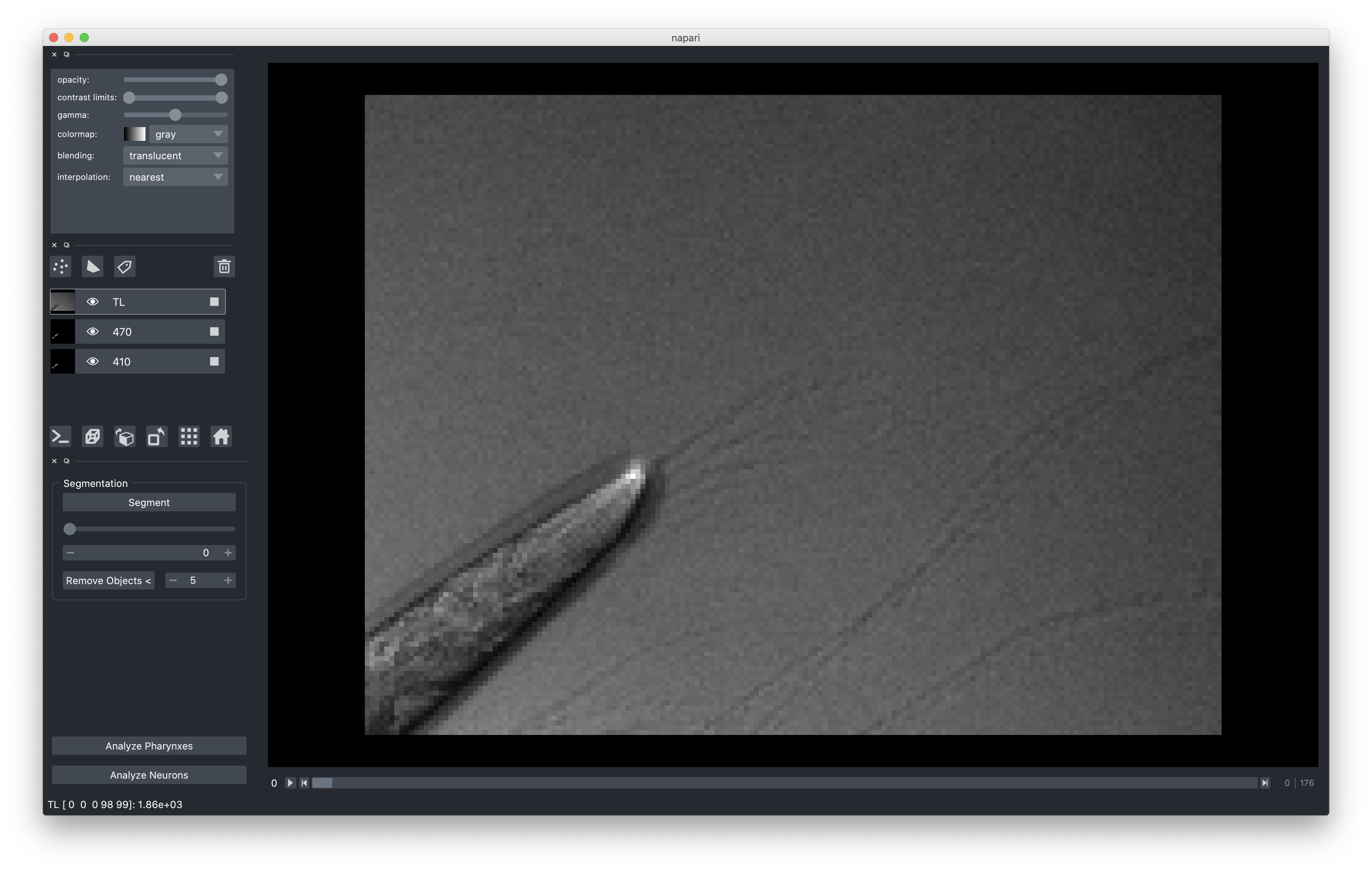
Set the threshold to a reasonable value based on your data. You can use the slider
or type in the threshold box to update the threshold interactively. If your images
contain small bright objects, you can use the Remove Objects < button to remove
objects smaller than the given number.
Once you are satisfied with the masks, simply press either Analyze Pharynxes or
Analyze Blobs, depending on your experiment. Analyze Blobs is meant for
measuring neurons, the gut, or any other structure with non-stereotypical geometry.
You can monitor the status of the pipeline through the terminal with which you
launched PhaRedox. If everything went well, there will be a pop-up window indicating
that the pipeline has finished running. When you click Open you will be taken to
the analysis directory containing the data from your experiment.
Getting at the Data
Each time you run an analysis, you will generate a directory within the analyses
directory. These subdirectories are named starting with the date on which the
analysis was run, and include a “strategy”, which was specified in your settings
file (this if for your reference, if you changed this or that setting you can come
up with a name to reflect that).
After running a single analysis, the directory structure will look something like this:
/Users/sean/Downloads/2019_05_16_gcy8_hsf1_afd_20C
├── 2019_05_16_gcy8_hsf1_afd_20C-indexer.csv
├── 2019_05_16_gcy8_hsf1_afd_20C.tif
├── analyses
│   └── 2020-04-16_testing
│       ├── 2019_05_16_gcy8_hsf1_afd_20C-trimmed_profile_data.csv
│       ├── 2019_05_16_gcy8_hsf1_afd_20C-trimmed_profile_data.nc
│       ├── 2019_05_16_gcy8_hsf1_afd_20C-trimmed_region_data.csv
│       ├── 2019_05_16_gcy8_hsf1_afd_20C-untrimmed_profile_data.csv
│       ├── 2019_05_16_gcy8_hsf1_afd_20C-untrimmed_profile_data.nc
│       ├── 2019_05_16_gcy8_hsf1_afd_20C-untrimmed_region_data.csv
│       └── figs
│           ├── 2019_05_16_gcy8_hsf1_afd_20C-movement_annotation_imgs.pdf
│           ├── 2019_05_16_gcy8_hsf1_afd_20C-ratio_images-pair=0;timepoint=0.pdf
│           └── profile_data
│               ├── trimmed_profiles
│               │   ├── avgs
│               │   │   ├── 2019_05_16_gcy8_hsf1_afd_20C-wavelength=410;pair=0;timepoint=0-avgs.pdf
│               │   │   ├── 2019_05_16_gcy8_hsf1_afd_20C-wavelength=470;pair=0;timepoint=0-avgs.pdf
│               │   │   ├── 2019_05_16_gcy8_hsf1_afd_20C-wavelength=e;pair=0;timepoint=0-avgs.pdf
│               │   │   ├── 2019_05_16_gcy8_hsf1_afd_20C-wavelength=oxd;pair=0;timepoint=0-avgs.pdf
│               │   │   └── 2019_05_16_gcy8_hsf1_afd_20C-wavelength=r;pair=0;timepoint=0-avgs.pdf
│               │   └── individual
│               │       ├── 2019_05_16_gcy8_hsf1_afd_20C-wavelength=410;pair=0;timepoint=0-individuals.pdf
│               │       ├── 2019_05_16_gcy8_hsf1_afd_20C-wavelength=470;pair=0;timepoint=0-individuals.pdf
│               │       ├── 2019_05_16_gcy8_hsf1_afd_20C-wavelength=e;pair=0;timepoint=0-individuals.pdf
│               │       ├── 2019_05_16_gcy8_hsf1_afd_20C-wavelength=oxd;pair=0;timepoint=0-individuals.pdf
│               │       └── 2019_05_16_gcy8_hsf1_afd_20C-wavelength=r;pair=0;timepoint=0-individuals.pdf
│               └── untrimmed_profiles
│                   ├── avgs
│                   │   ├── 2019_05_16_gcy8_hsf1_afd_20C-wavelength=410;pair=0;timepoint=0-avgs.pdf
│                   │   ├── 2019_05_16_gcy8_hsf1_afd_20C-wavelength=470;pair=0;timepoint=0-avgs.pdf
│                   │   ├── 2019_05_16_gcy8_hsf1_afd_20C-wavelength=e;pair=0;timepoint=0-avgs.pdf
│                   │   ├── 2019_05_16_gcy8_hsf1_afd_20C-wavelength=oxd;pair=0;timepoint=0-avgs.pdf
│                   │   └── 2019_05_16_gcy8_hsf1_afd_20C-wavelength=r;pair=0;timepoint=0-avgs.pdf
│                   └── individual
│                       ├── 2019_05_16_gcy8_hsf1_afd_20C-wavelength=410;pair=0;timepoint=0-individuals.pdf
│                       ├── 2019_05_16_gcy8_hsf1_afd_20C-wavelength=470;pair=0;timepoint=0-individuals.pdf
│                       ├── 2019_05_16_gcy8_hsf1_afd_20C-wavelength=e;pair=0;timepoint=0-individuals.pdf
│                       ├── 2019_05_16_gcy8_hsf1_afd_20C-wavelength=oxd;pair=0;timepoint=0-individuals.pdf
│                       └── 2019_05_16_gcy8_hsf1_afd_20C-wavelength=r;pair=0;timepoint=0-individuals.pdf
├── processed_images
│   ├── fluorescent_images
│   │   ├── 2019_05_16_gcy8_hsf1_afd_20C-wvl=410_pair=0.tif
│   │   ├── 2019_05_16_gcy8_hsf1_afd_20C-wvl=470_pair=0.tif
│   │   └── 2019_05_16_gcy8_hsf1_afd_20C-wvl=TL_pair=0.tif
│   ├── rot_fl
│   │   ├── 2019_05_16_gcy8_hsf1_afd_20C-wvl=410_pair=0.tif
│   │   ├── 2019_05_16_gcy8_hsf1_afd_20C-wvl=470_pair=0.tif
│   │   └── 2019_05_16_gcy8_hsf1_afd_20C-wvl=TL_pair=0.tif
│   ├── rot_seg
│   │   ├── 2019_05_16_gcy8_hsf1_afd_20C-wvl=410_pair=0.tif
│   │   ├── 2019_05_16_gcy8_hsf1_afd_20C-wvl=470_pair=0.tif
│   │   └── 2019_05_16_gcy8_hsf1_afd_20C-wvl=TL_pair=0.tif
│   └── segmented_images
│       ├── 2019_05_16_gcy8_hsf1_afd_20C-wvl=410_pair=0.tif
│       ├── 2019_05_16_gcy8_hsf1_afd_20C-wvl=470_pair=0.tif
│       └── 2019_05_16_gcy8_hsf1_afd_20C-wvl=TL_pair=0.tif